[经济学]第六章习题讲解计量经济学
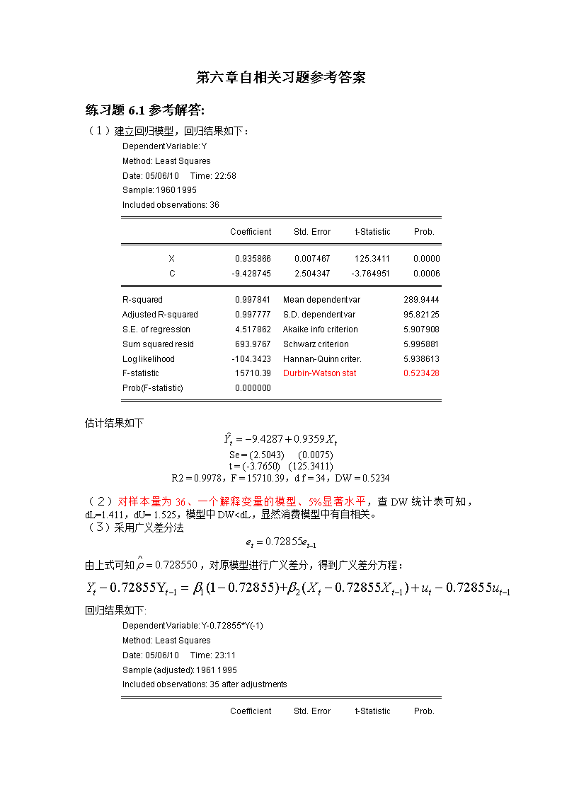
第六章自相关习题参考答案练习题6.1参考解答:(1)建立回归模型,回归结果如下:DependentVariable:YMethod:LeastSquaresDate:05/06/10Time:22:58Sample:19601995Includedobservations:36CoefficientStd.Errort-StatisticProb. X0.9358660.007467125.34110.0000C-9.4287452.504347-3.7649510.0006R-squared0.997841 Meandependentvar289.9444AdjustedR-squared0.997777 S.D.dependentvar95.82125S.E.ofregression4.517862 Akaikeinfocriterion5.907908Sumsquaredresid693.9767 Schwarzcriterion5.995881Loglikelihood-104.3423 Hannan-Quinncriter.5.938613F-statistic15710.39 Durbin-Watsonstat0.523428Prob(F-statistic)0.000000估计结果如下Se=(2.5043)(0.0075)t=(-3.7650)(125.3411)R2=0.9978,F=15710.39,df=34,DW=0.5234(2)对样本量为36、一个解释变量的模型、5%显著水平,查DW统计表可知,dL=1.411,dU=1.525,模型中DW
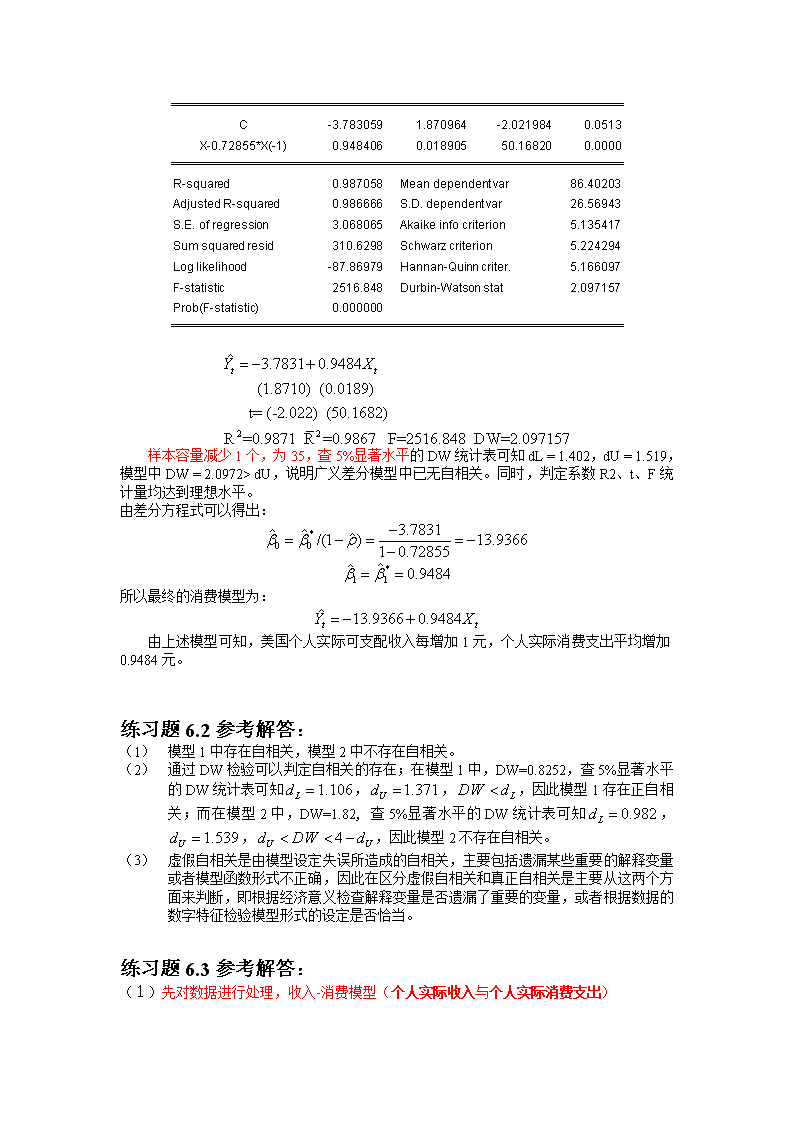
dU,说明广义差分模型中已无自相关。同时,判定系数R2、t、F统计量均达到理想水平。由差分方程式可以得出:所以最终的消费模型为:由上述模型可知,美国个人实际可支配收入每增加1元,个人实际消费支出平均增加0.9484元。练习题6.2参考解答:(1)模型1中存在自相关,模型2中不存在自相关。(2)通过DW检验可以判定自相关的存在;在模型1中,DW=0.8252,查5%显著水平的DW统计表可知,,,因此模型1存在正自相关;而在模型2中,DW=1.82,查5%显著水平的DW统计表可知,,,因此模型2不存在自相关。(3)虚假自相关是由模型设定失误所造成的自相关,主要包括遗漏某些重要的解释变量或者模型函数形式不正确,因此在区分虚假自相关和真正自相关是主要从这两个方面来判断,即根据经济意义检查解释变量是否遗漏了重要的变量,或者根据数据的数字特征检验模型形式的设定是否恰当。练习题6.3参考解答:(1)先对数据进行处理,收入-消费模型(个人实际收入与个人实际消费支出)\n个人实际消费支出=人均生活消费支出/商品零售物价指数*100建立回归模型,回归结果如下:DependentVariable:YMethod:LeastSquaresDate:05/06/10Time:23:20Sample:20012019Includedobservations:19CoefficientStd.Errort-StatisticProb. X0.6904880.01287753.620680.0000C79.9300412.399196.4463900.0000R-squared0.994122 Meandependentvar700.2747AdjustedR-squared0.993776 S.D.dependentvar246.4491S.E.ofregression19.44245 Akaikeinfocriterion8.872095Sumsquaredresid6426.149 Schwarzcriterion8.971510Loglikelihood-82.28490 Hannan-Quinncriter.8.888920F-statistic2875.178 Durbin-Watsonstat0.574663Prob(F-statistic)0.000000估计结果如下(2)DW=0.575,对样本量为36、一个解释变量的模型、5%显著水平的DW统计表可知,说明误差项存在正自相关。(3)采用广义差分法使用普通最小二乘法估计的估计值,得由上式可知=0.657352,对原模型进行广义差分,得到广义差分方程:回归结果如下:DependentVariable:Y-0.657352*Y(-1)Method:LeastSquares\nDate:05/06/10Time:23:25Sample(adjusted):20022019Includedobservations:18afteradjustmentsCoefficientStd.Errort-StatisticProb. C35.977618.1035464.4397370.0004X-0.657352*X(-1)0.6686950.02064232.395120.0000R-squared0.984983 Meandependentvar278.1002AdjustedR-squared0.984044 S.D.dependentvar105.1781S.E.ofregression13.28570 Akaikeinfocriterion8.115693Sumsquaredresid2824.158 Schwarzcriterion8.214623Loglikelihood-71.04124 Hannan-Quinncriter.8.129334F-statistic1049.444 Durbin-Watsonstat1.830746Prob(F-statistic)0.000000估计结果如下DW=1.830,已知,模型中因此,在广义差分模型中已无自相关。由差分方程式可以得出:(错误)(正确)因此,修正后的回归模型应为由上述模型可知,个人实际收入每增加1元,个人实际支出平均增加0.668695元。6.4参考答案1.原题(1)建立回归模型,回归结果如下:DependentVariable:Y\nMethod:LeastSquaresDate:11/26/10Time:19:47Sample:19701994Includedobservations:25CoefficientStd.Errort-StatisticProb. X1.5297120.05097630.008460.0000C-68.1602615.26513-4.4650960.0002R-squared0.975095 Meandependentvar388.0000AdjustedR-squared0.974012 S.D.dependentvar43.33397S.E.ofregression6.985763 Akaikeinfocriterion6.802244Sumsquaredresid1122.420 Schwarzcriterion6.899754Loglikelihood-83.02805 Hannan-Quinncriter.6.829289F-statistic900.5078 Durbin-Watsonstat0.348288Prob(F-statistic)0.000000给定n=25,,在的显著水平下,查DW统计表可知,。模型中,所以可以判断模型中存在正自相关。(2)对模型的修正1)采广义差分法修正自相关:使用普通最小二乘法估计的估计值,得由上式可知=0.873772,对原模型进行广义差分,得到广义差分方程:回归结果如下:DependentVariable:Y-0.873772*Y(-1)Method:LeastSquaresDate:11/26/10Time:20:04Sample(adjusted):19711994Includedobservations:24afteradjustmentsCoefficientStd.Errort-StatisticProb. X-0.873772*X(-1)1.2520330.1877946.6670590.0000C3.1980657.7907390.4104960.6854R-squared0.668922 Meandependentvar54.86397AdjustedR-squared0.653873 S.D.dependentvar6.671848\nS.E.ofregression3.925217 Akaikeinfocriterion5.652375Sumsquaredresid338.9612 Schwarzcriterion5.750547Loglikelihood-65.82850 Hannan-Quinncriter.5.678420F-statistic44.44968 Durbin-Watsonstat1.322343Prob(F-statistic)0.000001给定n=24,,在的显著水平下,查DW统计表可知,。模型中,DW值落在了无法判断的区域。所以修正后的模型为:2)一阶差分法对模型进行一阶差分,回归结果如下:DependentVariable:Y-Y(-1)Method:LeastSquaresDate:11/26/10Time:20:37Sample(adjusted):19711994Includedobservations:24afteradjustmentsCoefficientStd.Errort-StatisticProb. X-X(-1)1.3333330.13142210.145430.0000R-squared0.652682 Meandependentvar6.208333AdjustedR-squared0.652682 S.D.dependentvar6.678839S.E.ofregression3.936084 Akaikeinfocriterion5.619023Sumsquaredresid356.3333 Schwarzcriterion5.668109Loglikelihood-66.42828 Hannan-Quinncriter.5.632046Durbin-Watsonstat1.591830给定n=24,,在的显著水平下,查DW统计表可知,。模型中,因此模型已不存在自相关。3)德宾两步法建立辅助回归方程,回归结果如下:DependentVariable:YMethod:LeastSquaresDate:11/26/10Time:20:43Sample(adjusted):19711994\nIncludedobservations:24afteradjustmentsCoefficientStd.Errort-StatisticProb. C-7.63364112.84334-0.5943660.5589X1.1726220.1885276.2199190.0000X(-1)-1.0062720.254581-3.9526660.0008Y(-1)0.8962550.1239097.2331720.0000R-squared0.992083 Meandependentvar391.6667AdjustedR-squared0.990896 S.D.dependentvar40.10927S.E.ofregression3.827019 Akaikeinfocriterion5.673061Sumsquaredresid292.9215 Schwarzcriterion5.869403Loglikelihood-64.07673 Hannan-Quinncriter.5.725151F-statistic835.4552 Durbin-Watsonstat1.369050Prob(F-statistic)0.000000把的回归系数看做的一个估计值,之后进行广义差分,回归模型为:回归结果如下:DependentVariable:Y-0.896255*Y(-1)Method:LeastSquaresDate:11/26/10Time:20:47Sample(adjusted):19711994Includedobservations:24afteradjustmentsCoefficientStd.Errort-StatisticProb. X-0.896255*X(-1)1.2010310.1893056.3444250.0000C4.6528996.5955020.7054660.4879R-squared0.646596 Meandependentvar46.19771AdjustedR-squared0.630532 S.D.dependentvar6.352384S.E.ofregression3.861224 Akaikeinfocriterion5.619501Sumsquaredresid327.9990 Schwarzcriterion5.717672Loglikelihood-65.43401 Hannan-Quinncriter.5.645545F-statistic40.25173 Durbin-Watsonstat1.305817Prob(F-statistic)0.000002给定n=24,,在的显著水平下,查DW统计表可知,。模型中,DW值落在了无法判断的区域。2.调换X和Y之后(1)建立回归模型,回归结果如下:\nDependentVariable:YMethod:LeastSquaresDate:12/04/10Time:11:21Sample:19701994Includedobservations:25CoefficientStd.Errort-StatisticProb. X0.6374370.02124230.008460.0000C50.874548.2910586.1360730.0000R-squared0.975095 Meandependentvar298.2000AdjustedR-squared0.974012 S.D.dependentvar27.97320S.E.ofregression4.509491 Akaikeinfocriterion5.926864Sumsquaredresid467.7167 Schwarzcriterion6.024374Loglikelihood-72.08580 Hannan-Quinncriter.5.953909F-statistic900.5078 Durbin-Watsonstat0.352762Prob(F-statistic)0.000000给定n=25,,在的显著水平下,查DW统计表可知,。模型中,所以可以判断模型中存在正自相关。(2)对模型的修正1)采广义差分法修正自相关:使用普通最小二乘法估计的估计值,得由上式可知=0.850961,对原模型进行广义差分,得到广义差分方程:回归结果如下:DependentVariable:Y-0.850961*Y(-1)Method:LeastSquaresDate:12/04/10Time:11:17Sample(adjusted):19711994Includedobservations:24afteradjustmentsCoefficientStd.Errort-StatisticProb. X-0.850961*X(-1)0.5351250.0747937.1547960.0000C13.973344.7894362.9175330.0080\nR-squared0.699417 Meandependentvar48.03762AdjustedR-squared0.685754 S.D.dependentvar4.550930S.E.ofregression2.551144 Akaikeinfocriterion4.790616Sumsquaredresid143.1833 Schwarzcriterion4.888787Loglikelihood-55.48739 Hannan-Quinncriter.4.816661F-statistic51.19110 Durbin-Watsonstat2.377660Prob(F-statistic)0.000000给定n=24,,在的显著水平下,查DW统计表可知,。模型中,因此可以判断模型不存在自相关。所以修正后的模型为:6.5参考解答:(1)建立回归模型,回归结果如下:DependentVariable:LOG(Y)Method:LeastSquaresDate:05/07/10Time:00:17Sample:19802000Includedobservations:21CoefficientStd.Errort-StatisticProb. C2.1710410.2410259.0075290.0000LOG(X)0.9510900.03889724.451230.0000R-squared0.969199 Meandependentvar8.039307AdjustedR-squared0.967578 S.D.dependentvar0.565486S.E.ofregression0.101822 Akaikeinfocriterion-1.640785Sumsquaredresid0.196987 Schwarzcriterion-1.541307Loglikelihood19.22825 Hannan-Quinncriter.-1.619196F-statistic597.8626 Durbin-Watsonstat1.159788Prob(F-statistic)0.000000\n给定n=21,,在的显著水平下,查DW统计表可知,。模型中,所以可以判断模型中存在正自相关。(2)采用广义差分法修正自相关:使用普通最小二乘法估计的估计值,得由上式可知=0.400234,对原模型进行广义差分,得到广义差分方程:回归结果如下:DependentVariable:LOG(Y)-0.400234*LOG(Y(-1))Method:LeastSquaresDate:05/07/10Time:00:21Sample(adjusted):19812000Includedobservations:20afteradjustmentsCoefficientStd.Errort-StatisticProb. C1.4770950.2256366.5463720.0000LOG(X)-0.400234*LOG(X(-1))0.9059890.05976715.158710.0000R-squared0.927357 Meandependentvar4.882162AdjustedR-squared0.923321 S.D.dependentvar0.344052S.E.ofregression0.095271 Akaikeinfocriterion-1.769534Sumsquaredresid0.163380 Schwarzcriterion-1.669961Loglikelihood19.69534 Hannan-Quinncriter.-1.750096F-statistic229.7864 Durbin-Watsonstat1.441543Prob(F-statistic)0.000000给定n=20,,在的显著水平下,查DW统计表可知,。模型中,所以可以判断广义差分模型中不存在自相关。由差分方程式可以得出:\n所以修正后的模型为:(3)变换数据后的回归结果如下:DependentVariable:LOG(Y/Y(-1))Method:LeastSquaresDate:05/07/10Time:00:23Sample(adjusted):19812000Includedobservations:20afteradjustmentsCoefficientStd.Errort-StatisticProb. C0.0540470.0133224.0568960.0007LOG(X/X(-1))0.4422240.0660246.6979010.0000R-squared0.713658 Meandependentvar0.091592AdjustedR-squared0.697750 S.D.dependentvar0.098311S.E.ofregression0.054049 Akaikeinfocriterion-2.903219Sumsquaredresid0.052583 Schwarzcriterion-2.803646Loglikelihood31.03219 Hannan-Quinncriter.-2.883781F-statistic44.86188 Durbin-Watsonstat1.590363Prob(F-statistic)0.000003给定n=20,,在的显著水平下,查DW统计表可知,。模型中,所以可以判断变化数据后的模型中不存在自相关。